Uncontrolled RDS Timezone File Auto-Upgrade

By Brian Fitzgerald

Summary

Oracle databases require consistent timezone file versions between the source and target databases during imports. If the source database has a higher timezone file version than the target, the target’s version must be upgraded. In Oracle on-premises environments, this requires direct OS access, which is not available in AWS RDS.

AWS provides the TIMEZONE_FILE_AUTOUPGRADE option to manage this automatically, but it can cause unexpected disruptions due to undocumented behaviors. Understanding these behaviors and managing them carefully is necessary to prevent unexpected DB instance reboots.

Background

Timezone rules change in response to societal preferences and political changes. These changes can include the timezone offset from UTC, daylight saving time (DST) start and end dates, adoption or repeal of DST, timezone names and abbreviations, and more.

Oracle Database uses the timezone file to interpret the timezone stored with timestamps in the timestamp with time zone data type. For example, in the following SQL command:

SELECT TO_TIMESTAMP_TZ('July 19, 1969 9:32 AM EDT',
'Month dd, yyyy hh:mi AM
tzd’) liftoff FROM dual;

Oracle determines that Eastern Daylight Time was 4 hours behind UTC in July 1969.

Ittoqqortoormiit, Greenland

When timezone rules change, the timezone file is updated to reflect the change and its effective date. For example, on March 31, 2024, Ittoqqortoormiit, Greenland, changed its timezone rules. Timestamps before this date are interpreted differently than those after it.

Oracle includes timezone file updates with quarterly patch release updates (RUs) if an updated file is available. Some RUs have no timezone file update. However, in Q1 2023, Oracle issued two RUs, each with a new timezone file update.

To upgrade the timezone file on-premises, download and run the MOS script upg_tzv_apply.sql, which starts your database in upgrade mode and runs the dbms_dst package.

The active timezone file version can be found by running:

select version
from v$timezone_file

AWS does not permit customers to directly start an RDS Oracle database in upgrade mode, so it offers the TIMEZONE_FILE_AUTOUPGRADE option. You can enable this option for one or more databases by adding it to the databases’ option group, or by switching a database to an option group with this option. Note that an option group applies to a single account, region, engine, and Virtual Private Cloud (VPC).

AWS states, “When the option group attached to your RDS for Oracle DB instance includes the TIMEZONE_FILE_AUTOUPGRADE option, RDS updates your time zone files automatically.” This statement hides undocumented behavior that first-time users may find counterintuitive.

Behavior

Once the TIMEZONE_FILE_AUTOUPGRADE option is enabled for a database, two conditions must be understood.

Whether the timezone file will be upgraded

You can determine if a timezone file will be upgraded by comparing the active version from v$timezone_file to the version found in the Amazon RDS for Oracle Release Notes. For instance, if your timezone file version is 42 and your engine version is 19.0.0.0.ru-2024-07.rur-2024-07.r1, RU 2024-07.ru did not change the timezone file version. However, the previous version, 19.0.0.0.ru-2024-04.rur-2024-04.r1, included “DSTV43”.

Conclusion: If TIMEZONE_FILE_AUTOUPGRADE is enabled, your DB engine version is 19.0.0.0.ru-2024-07.rur-2024-07.r1, and your timezone file version is 42, the file will be automatically upgraded. Identifying the highest available version requires reviewing the documentation.

When the timezone file will be upgraded

If the timezone file will be upgraded. the upgrade occurs:

  1. During the next maintenance window, or
  2. Immediately, if any immediate change is made to the DB instance.

The immediate upgrade is undocumented and can cause unexpected behavior. The database will reboot and upgrade the timezone file if you make any immediate changes, such as changing:

  1. Maintenance window
  2. Backup window
  3. Deletion protection
  4. IOPS or storage throughput
  5. CA Certificate identifier
  6. Auto minor version upgrade
  7. Master user password

Example scenario

Suppose you had created an Oracle EE RDS DB instance in 2022 with the following settings:

  1. DB Engine version:19.0.0.0.ru-2022-01.rur-2022-01.r1
  2. Timezone file version: 37
  3. Preferred maintenance window: Saturday 06:00 to 07:00
  4. Auto minor version upgrade: Enabled

By 2024, the DB Engine version is 19.0.0.0.ru-2024-04.rur-2024-04.r1 and timezone file version 43 is available.

If, say, on June 5, 2024, you add the TIMEZONE_FILE_AUTOUPGRADE option, no “pending” changes appear in the AWS console. However, if on June 17, you change storage throughput, the DB instance will reboot and apply the timezone file version change.

Immediate upgrade behavior only happens if the active timezone file version is less than the available version.

Discussion

Most RDS DB instance attributes can be checked and modified by running describe-db-instances and modify-db-instance. Other modifications can be made using option groups, parameter groups, or maintenance actions. However, controlling the timezone file version differs.

To check for a pending timezone file upgrade, examine v$timezone_file and your DB engine version documentation. There is no direct indication of an upgrade pending.

You cannot issue a command that directly upgrades a timezone file version. The TIMEZONE_FILE_AUTOUPGRADE and database upgrades must be implemented carefully, as many unrelated commands can inadvertently trigger an immediate upgrade and reboot.

Internal Process

If TIMEZONE_FILE_AUTOUPGRADE is enabled, any immediate or scheduled DB instance change prompts the hypervisor to connect via cloud-init and compare active and available timezone file versions. If a newer version is available, cloud-init restarts the database in upgrade mode and runs dbms_dst to upgrade the file version.

Documentation

The apparent spontaneous reboot behavior is not documented.

Workaround

One workaround is to not use the TIMEZONE_FILE_AUTOUPGRADE option. However, this choice limits flexibility across imports. A better option is to keep the option enabled, ensuring timezone files are updated with DB instance upgrades.

If implementing TIMEZONE_FILE_AUTOUPGRADEon an existing DB instance, do so just before the next version upgrade and avoid further modifications until the upgrade is complete.

“Master Arm is On”

One minute before liftoff from the Moon in the Apollo 11 Lunar Module ascent stage, Neil Armstrong activated the Master Arm switch. When the countdown clock reached zero, a complex sequence of events unfolded: pyrotechnics separated the ascent stage electrically and mechanically from the descent stage and opened explosive helium pressurization valves to prepare for ascent stage engine ignition. The purpose of the “arming switch” is, therefore, to enable an intentional, automatic, sequenced operation of circuits, actuators, and firing of pyrotechnics in the ascent stage launch sequence. Apollo 11 Lunar Module ascent stage

The TIMEZONE_FILE_AUTOUPGRADE option functions like an arming switch. Once set, the timezone file upgrade is “armed”. The normal actuating trigger is a DB instance engine upgrade. However, any DB instance change will also trigger the timezone file upgrade.

Our DBA team enabled TIMEZONE_FILE_AUTOUPGRADE on a Friday morning, with a minor version upgrade scheduled for the following maintenance window. We adopted the custom of announcing, “Master Arm is On,” indicating team members should refrain from ad-hoc, immediate changes until after the engine and timezone file upgrade.

During the maintenance window, both the DB engine and timezone file versions were upgraded. The TIMEZONE_FILE_AUTOUPGRADE option remained enabled for future updates.

We experienced no issues or surprises in production, development, or QA environments. All abnormal behavior was identified during testing, and implementation was coordinated to avoid adverse effects.

Conclusion

Maintaining synchronization of the timezone file version is crucial for import flexibility. The TIMEZONE_FILE_AUTOUPGRADE option automates upgrades but requires careful handling to avoid unexpected outages.

Elastic Block Store throughput testing with Orion

By Brian Fitzgerald

Introduction

ORacle I/O Numbers (Orion) results for EBS volumes are presented here. Multiple configurations of EC2 instance type, number of devices, IOPS configuration, and throughput configuration are tested. The objective is to identify the best performing and most economical system for use in Oracle Automatic Storage Management (ASM).

Amazon AWS EC2 EBS

AWS EC2 offers I/O capacity for a price. You get a slice of the underlying hardware’s full bandwidth depending on how much you pay. The actual throughput depends on the EC2 instance’s device controller and the underlying volume. EC2 device controller capacity depends on instance class (m5, r5b, etc.), and size (large, 4xlarge, etc.). EBS volume capacity depends on volume type (gp3, io2, etc.) and configuration (throughput and IOPS). Maximum I/O capacity will be the lesser of EC2 capacity and EBS volume capacity, provided that you get the layout right.

The I/O capabilities of the EBS volume types that were tested are summarized here:

Type gp3 gp2 st1 io2
Purpose General General Low cost High IOPs, low latency
Medium ssd ssd magnetic ssd
Configurable throughput Yes No No No
Maximum throughput configuration (Mbps) 1000 – – –
Configurable IOPS Yes Yes
Max IOPS configuration 160000 256,000

The EBS test volumes were not encrypted.

This article places emphasis on optimizing throughput, but some IOPS and latency observations are presented here as well. As a limiting case, we are interested in 100% write I/O throughput capacity.

I/O throughput rating on EC2

We are mainly concerned with the modern, Nitro EC2 m5, c5, r5, and r5b instance types. Throughput is defined as the rate, in Mbps for large (128 KiB) I/O, and could refer to a read, write, or mixed (read-write) workload.

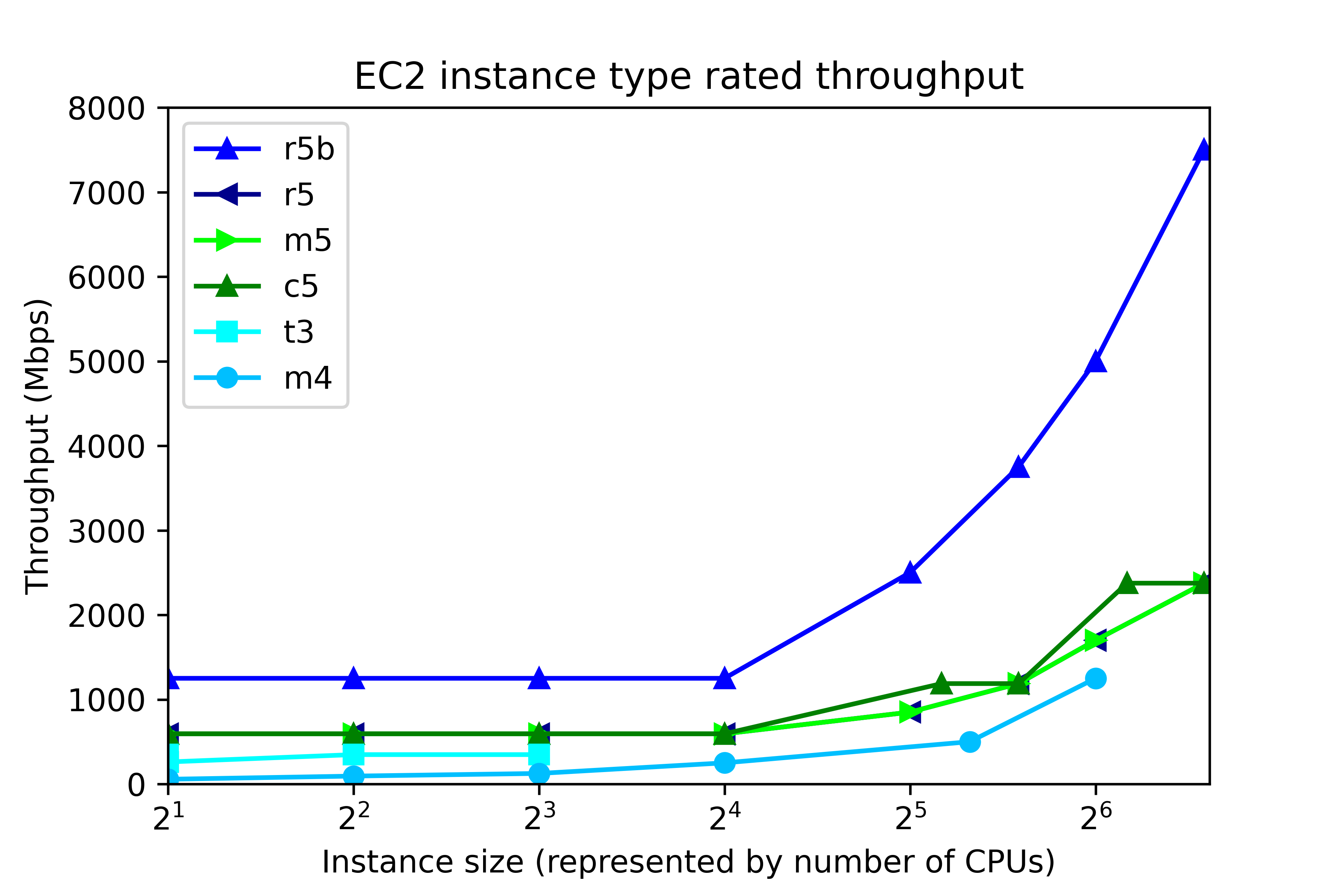
EC2 throughput rating can be found by running “aws ec2 describe-instance-types”, and is divided into two ranges, according to instance size, as shown in the following figure. The number of CPUs in EC2 maps to instance size thus:

Number of CPUs Instance size
2 large
4 xlarge
8 2xlarge
16 4xlarge
32 8xlarge
48 12xlarge
64 16xlarge
96 24xlarge

At the low end, up to 4xlarge, throughput is capped at a single value, regardless of instance size. That cap depends on instance class. In r5b, the cap is 1250 Mbps, but for c5, m5, and r5, throughput is capped at 593.75 Mbps. Other instance classes have lower throughput caps. At the high end, 8xlarge and up, throughput depends on the instance size. The r5b instance class tops out at 7500 Mbps. m5, c5, and r5 classes have throughput that ranges from 850 Mbps to 2375 Mbps, depending on instance type.

By now we have described the available volume types and instance types. So let’s pose this question. If we configure 8 gp3 volumes at 1000 Mbps each, then the system should deliver 8000 Mbps throughput, right?

Wrong.

No EC2-EBS-Linux system today delivers 8000 Mbps throughput. You will get, at best, the throughput offered by the EC2 instance type. For example, if you build an m5.4xlarge instance, then the highest possible throughput will be 593.75 Mbps, as I mentioned. Also, 593.75 Mbps is the most you will get. Actually achieving that requires configuring multiple volumes.

Operating system description

The test system is an Amazon AWS EC2 instance running Red Hat Linux 7.9. The test software is orion, which is found in the Oracle home. The number of CPUs, the amount of memory, and the device controller interface depend on the EC2 instance type. For example, the m5.xlarge has 4 CPUs, 16 GB RAM, and a non-volatile memory express (NVMe) device controller interface.

Test description

100% write I/O was tested with orion. General purpose volumes (gp2 and gp3), and the lower cost st1 storage were tested with large writes. I/O optimized storage (io2) was tested at small I/O. Each test ran from 4 to 20 minutes, depending on the number of volumes. For the throughput tests, “Maximum Large MBPS” was extracted from the summary.txt file. In the small I/O tests, “Maximum Small IOPS” and “Minimum Small Latency” were extracted.

Instance type and volume type

In this section, the influence of instance type and volume type in investigated. The new I/O-optimized r5b instance type was tested with gp3 storage. General purpose m5 instance class was tested with gp2, gp3, and io2 storage. Additionally, the lower cost, burstable t3 instance class, and the previous generation m4 instance class were tested. The number of CPUs ranged from 2 to 96. As a rule of thumb, the amount of memory for the m5, t3, and m4 instance classes, in GB, is four times the number of CPU. Eight 125-GB volumes were tested in every run. In all, there were 31 test runs.

Throughput testing

General  purpose storage was tested for throughput. gp3 storage was configured for 1000 Mbps throughput per volume (the maximum) and 4000 IOPS The results are displayed here.Each point represents the maximum throughput obtained in a single test. The dark blue line, for example, displays Orion throughput results for 6 tests on r5b.large, r5b.4xlarge, r5b.8xlarge, r5b.12xlarge, r5b.16xlarge, r5b.24xlarge, The test points above 24 are results of separate tests on r5b.4xlarge, m5.4xlarge on gp3 volume type, m5.4xlarge on gp2 volume type, t3.4xlarge, m4.4xlarge, and m5.4xlarge on st1 volume type. Again, each point is a separate test, not Orion data points from a single test.

The figure shows actual system throughput for 8 volumes. We already said that just because you configure 8 1000 Mbps volumes does not mean that the observed throughput will be 8000 Mbps. Instead, the throughput is limited by the instance type.

The key points to notice in the throughput testing are:

  • The observed throughput is level across instance types up to 4xlarge (24 CPUs), just like the documentation says.
  • Starting at 8xlarge, (25 CPUs), gp3 throughput scales up with the instance size, reaching 7330 Mbps on the r5b.24xlarge instance type, and 2330 Mbps on m5.24xlarge, again, just like the documentation says.
  • Like gp3 on the m5, gp2 throughput is level at 580 Mbps for instances up to 4xlarge.
  • From 12xlarge and up, gp2 throughput is level at 1015 MPBs.
  • For t3.xlarge and up, throughput plateaus at 335 Mbps.
  • In older instance class m4, throughput ranges from 55 Mbps to 240 Mbps.

Notice that in high-end instance types, r5b throughput is better than 3x the m5 throughput. This is one example where actual observations match the marketing materials: New – Amazon EC2 R5b Instances Provide 3x Higher EBS Performance

By using the number of CPUs on the horizontal axis, we do not mean to imply that CPUs have a significant influence on system throughput in EC2. In fact, during ORION testing, CPU workload tends be low, and the same can be said for memory footprint. Plotting vs “Number of CPUs” is just meant to be a convenient method for having plotting I/O numbers vs instance size. AWS throttles throughput depending on instance type and size, separately from the number of CPUs.

IOPS testing

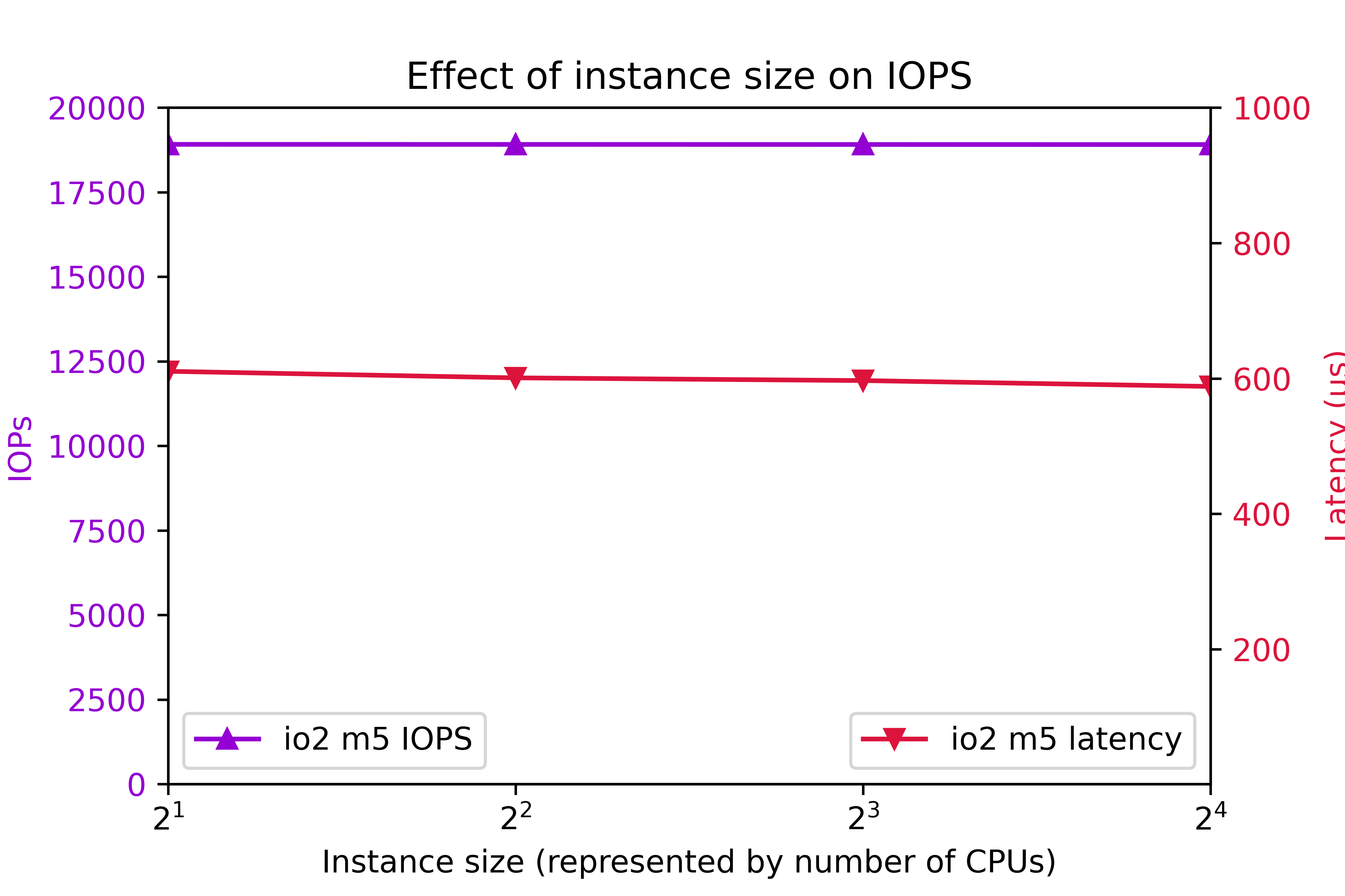
I/O Optimized storage io2 configured for 7000 IOPS per volume on the m5 class was also tested. 8 volumes were tested.Again, to clarify, configured IOPS for each volume was 7000. You might think that configuring 8 volumes are 7000 IOPS per volume should deliver 56000 IOPS. As you can see, actual IOPS is less.

The key IOPS testing observations are:

  • IOPs is flat at 18905.
  • Latency is flat at 600ms.

Conclusion

  • r5b throughput outperforms m5 by better than 3x.
  • I/O performance is level up to 4xlarge.
  • Starting at 8xlarge, throughput ramps up with instance class.
  • 24xlarge delivers the highest throughput.
  • t3 write throughput lags m5, and m4 write throughput lags t3.
  • The observed system I/O rate is much less than you would expect if you calculated I/O rate based on the volume configuration.

This section was an overview of the capabilities of various EC2 instance types and volume types with eight volumes. As we are about to see, tuning the number of volumes is crucial to optimizing instance performance.

Number of volumes

The influence of the number of volumes on I/O was tested for various instance types. The number of volumes ranged from 1 to 16. Throughput was tested on general purpose volume types gp2 and gp3. The gp3 storage was configured for 1000 Mbps and 4000 IOPs per volume. The results are shown in the following figure:Additionally, IOPS was measured on on I/O optimized volume type io2. IOPS was set at 7000 per volume. The results are shows here:The key findings are

  • For improved throughput, I/O should be distributed across multiple volumes.
  • In r5b.24xlarge, throughput increases all the way out to 7300 Mbps at 16 volumes.
  • In r5b8xlarge and m5.24xlarge, throughput levels off around 2400 Mbps at 8 volumes.
  • On m5.large, gp2 and gp3 throughput levels off at 580 Mbps at four volumes.
  • On m5.large, io2 IOPs plateaus at 18905 IOPs at four volumes.
  • io2 latency tends to remain below 625ms.

Be aware that the EC2 device attachment limit is 28, including the network adapter and up to 27 volumes, including the system disk. A practical Oracle ASM system could consist of two diskgroups and four or more disks per group.

In conclusion, one can expect improve I/O by implementing four volumes. In high end systems, configuring eight or more volumes is beneficial. Exercise prudence on the number of volumes, because throughput and IOPS charges are per-volume.

Configured volume throughput

So far, we have tested volumes that are over-provisioned, meaning that measured throughput turned out to be much less than rated throughput. You don’t get what you pay for. So how much throughput should you actually be configuring?

In this section, we investigate the effect of configured throughput versus actual throughput on gp3 volumes. gp3 volumes were configured at 3000 IOPs and a throughput range from 125 Mbps to 1000 Mbps. Various m5 and r5b instance types were tested. The results are shown here.In the m5.large, m5.24xlarge, and r5b.8xlarge cases, setting volume throughput to 375 Mbps achieves the maximum possible system throughput. Setting volume throughput higher than that leads to no further gains in performance. In r5b.12xlarge and r5b.24xlarge, performance can be maximized by setting throughput to 500 Mbps. In conclusion, although gp3 throughput can be adjusted to 1000 Mbps, there is no benefit to setting gp3 throughput above 500 Mbps, and only in rare cases is it beneficial to set gp3 throughput above 375 Mbps.

Intel vs. AMD

AWS offers a choice of Intel or AMD processor on Red Hat EC2. AMD EC2 prices are 10% lower than Intel. Rated EBS throughput on the AMD systems is less than on Intel.

AMD
Intel
instance type throughput (Mbps) instance type throughput (Mbps)
t3a.medium t3.medium
m5a.large 2880 m5.large 4750
m5a.24xlarge 13570 m5.24xlarge 19000

The test system configurations were:

Instance type CPUs Volumes Storage Throughput IOPS
t3[a].medium 2 4 st1 –
m5[a].large 2 8 gp3 375 3000
m5[a].24xlarge 96 8 gp3 375 3000

“t3[a].medium” refers to a comparison of a t3a.medium (AMD) system to a t3.medium (Intel) system, and so on, for m5[a].large and m5[a].24xlarge.At the low end instance types, AMD and Intel performed equally. At the high end, Intel edged AMD.

Systems for different purposes

Recommendations for three different type of systems are presented here. The target system is Oracle Database on top of Grid Infrastructure on Red Hat. Only systems with at least 2 CPUs and 4 GB RAM are considered. A “system” could refer to an ASM diskgroup, such as DATA, RECO, or REDO.

Low cost

You might need a low cost system for light development, well-tuned reports, archiving, etc. Use the t3a instance class and st1 storage.

General purpose

For general purpose production systems, use the m5 class. If you want to halve the memory, substitute c5 and save 9% to 11%. To double the system memory, use r5 and pay 24% to 30% more. Configure four or more gp3 volumes per ASM diskgroup at 125 Mbps to 375 Mbps throughput and 3000 IOPS.

High throughput

For highest large write throughput on EBS, use r5b.24xlarge, and at 16 gp3 volumes configured at 500 Mbps.

Example systems and cost

Example of the three types of system are presented in this table. This time, we present CPU and storage cost, assuming Red Hat Linux and on demand pricing in region us-east-1, as of 7/24/2021.

Purpose Instance Type Vol type Num CPU Vol Size Num Vols Thr IOPS Actual Mbps EC2 EBS Total
Low cost t3a.medium st1 2 125 8 – – 245 $71 $45 $116
General purpose m5.large gp3 2 250 4 125 3000 497 $114 $80 $194
High throughput r5b.24xlarge gp3 96 1000 16 500 3000 7330 $5316 $1522 $6838

Do not waste money

Follow this guidance to avoid wasting money

  • Avoid io2 EBS for general purpose Oracle databases. The cost is prohibitive.
  • In gp3, configure throughput at 500 Mbps or less, and configure 3000 IOPS.
  • For good, economical performance, configure gp3 at 125 Mbps and 3000 IOPS.

Workload

This article offers guidance on configuring the AWS EBS at 100% write. The findings apply to any diskgroup, particularly to redo diskgroups and to databases with high throughput requirements, such as ETL systems. The information is among many factors to consider when specifying a practical database system. Orion is also capable of simulating a 100% read workload, and a mixed workload. Mixed workload Orion results could be used to look for further cost reductions. Actual database application performance depends not only on storage throughput, but also on processor design, amount and speed of memory, and table design.

ASM diskgroup layout

Oracle makes ASM diskgroup layout recommendations: RAC and Oracle Clusterware Best Practices and Starter Kit (Platform Independent) (Doc ID 810394.1).

Oracle recommends a minimum 4 disks per diskgroup:My own test results show that a minimum of 4 LUNs per diskgroup lead to optimal throughput. Configuring 4 or more LUNs per diskgroup is extremely important.

Oracle recommends no more than 2 ASM diskgroups:Benefits of no more than 2 ASM diskgroups:

  • Simplified administration.
  • High throughput in all diskgroups.
  • Avoid approaching the EC2 attachment limit.

If you configure more than 2 diskgroups, you could find yourself making design compromises at exactly the wrong places. For example, online redo logs are critical, high throughput components. If you configure separate REDO diskgroups in EC2, then you may find it difficult to keep to 4 disks per diskgroup, and still allow for expansion and remain within the attachment limit. Or you may find that so many diskgroups leads to a manageability issue.

Conclusion

The r5b instance class with gp3 storage delivers the highest performing I/O. m5, c5, and r5 instance classes make well-performing, general purpose systems with high throughput. The t3a instance class with st1 storage makes a fair-performing, low cost system. Each ASM disk groups should be configured with a minimum of 4 disks and more than 4 disks for high throughput r5b systems. For optimal throughput, gp3 EBS should be configured at 3000 IOPS and no more than 500 Mbps.

Connecting across VPCs using Peering

By Brian Fitzgerald

Introduction

The requirement to connect applications across regions is ubiquitous. In Amazon Web Services (AWS), applications are deployed to a Virtual Private Cloud (VPC), but a VPC is specific to a single AWS region — to connect across regions, it is necessary to connect across VPCs. For speed and security, it is preferable to connect VPCs across Amazon’s internal networks, not across the public internet. We are going to establish our cross-VPC connection using peering. For this peering to succeed, planning is necessary to avoid overlapping IP address ranges. Peering across AWS accounts will also be demonstrated.

Virtual Private Clouds

An Amazon AWS Virtual Private Cloud (VPC) is an isolated network in a single region. A VPC covers all availability zones in the region and can have multiple subnets. A VPC covers a specific CIDR (Classless Inter-Domain Routing) IP address range, or “block”. In this section, we’re going to cover VPC IP address ranges, which is going to lead into the next section on VPC peering.

Networks

IP network configuration in AWS VPCs is quite flexible. The network number can reflect almost any legal IPv4 address range. IPv6 CIDR ranges are also available. A VPC CIDR block size can range from /16 netmask (65534 IP addresses) to /28 netmask (14 IP addresses).

Amazon recommends that you specify a CIDR block from the private IPv4 address ranges as specified in RFC 1918:

  • 10.0.0.0 – 10.255.255.255 (10/8 prefix)
  • 172.16.0.0 – 172.31.255.255 (172.16/12 prefix)
  • 192.168.0.0 – 192.168.255.255 (192.168/16 prefix)

If you use an AWS tool to automatically create a VPC, you will find that the generated CIDR follows that guidance. Here are some examples of VPC CIDR blocks generated by AWS tools:

  • 10.0.0.0/16
  • 172.31.0.0/16

You may create a VPC with a CIDR block outside the RFC 1918 ranges, but most users will refrain from doing so on aesthetic grounds, or to avoid misunderstandings. You may not create an AWS VPC CIDR block beginning with 0. or 127.

The default limit on VPCs is 5 = per region. To get a higher limit, you have to open a support case and submit a limit increase request. To avoid needing a higher VPC limit, you might decide to create your VPCs as large as allowable, i.e. netmask /16, and to avoid inadvertently creating ones. Some AWS only work by creating a new VPC. For example, if you use the Getting Started menu to setup an Elastic Container Service with load balancing, you will have no option but to create a new VPC. Other AWS tools offer to create a new VPC For example if you create a new a new EC2 or RDS instance in the AWS console, the menu offers creating a new VPC as as option. In conclusion, you can tightly manage your number of VPCs, or you can request a higher limit.

One way to simplify and standardize your administration is to create all your VPCs using RFC 1918 IP address ranges and netmask /16. If you do that, you can create networks among these ranges

  • 10.0.0.0/16 – 10.255.0.0/16 (256 networks)
  • 172.16.0.0/16 – 172.31.0.0/16 (16 networks)
  • 196.168.0.0/16 (1 network)

for a total of up to 273 VPCs per region. For many applications, 273 VPCs per region is ample.

In a new account, the default VPC in each region has CIDR block 172.31.0.0/16. As of this writing, a new account covers 17 regions. The upshot is that a new AWS account has 17 VPCs all with the same CIDR block. In the case of isolated VPCs, this is not a problem, but default VPCs cannot be connected by peering because the IP address ranges overlap.

In addition to creating new VPCs, you can increase the size of an existing VPC by adding additional CIDR blocks. However, you cannot mix across RFC 1918 IP address ranges. Specifically, you cannot combine “10.0” and “172.” CIDR blocks in a single VPC.

In conclusion, if you consider all allowable ranges and netmasks, you can choose from over a half billion possible CIDR blocks. However, even if you restrict your choice to private networks and the largest allowable size, you can choose from among 273 different CIDR blocks.

Subnets

Subnetting VPCs is also quite flexible. You may specify a subnet mask ranging from /16 (65534 IP addresses) to /28 (14 IP addresses). By default, a VPC may have up to 200 subnets.

You cannot create a subnet larger than netmask /16. For example, if you compose a VPC from two contiguous netmask /16 networks, you could not, therefore, create a single netmask /15 subnet.

VPC summary

A new account covers multiple regions, each with a default VPC with CIDR block range 172.31.0.0/16. You can create additional VPCs. Some users may decide to stick with netmask /16 and RFC 1918 networks. The detailed explanations of VPC IP addresses in this section set the stage for the next section, which is VPC peering.

VPC Peering

A simple way to connect across VPCs is to establish VPC peering. VPC peering connects two VPCs to form a single network. Traffic is routed not across the Internet, but across a private AWS network. VPC peering is more secure and more reliable than using an internet gateway.

VPC peering requires that the VPC CIDR blocks do not overlap. Subnets are not considered. In other words, if two VPCs have overlapping CIDRs, you cannot establish VPC peering, even if no existing subnets overlap.

All default VPC CIDR blocks are 172.31.0.0/16. You cannot establish VPC peering across more than one default VPC because the IP address range overlaps. You must create one or more new VPC.

For this blog, we’re going to setup VPC peering across regions us-east-1, ap-northeast-1, and eu-west-1 (N. Virginia, Tokyo, and London). We’ll start by deleting the default VPC, namely 172.31.0.0/16, and creating these VPCs

Region Region VPC ID CIDR block
N. Virginia us-east-1 vpc-0ed2447f33a01d301 10.1.0.0/16
Tokyo ap-northeast-1 vpc-07251b9829e270787 10.2.0.0/16
London eu-west-2 vpc-0bf90b5507089c175 10.3.0.0/16

For example:

vpc

I have deleted the default VPCs for neatness: I have no need for them now. In each new VPC, create a subnet. Also, only for the sake of this blog, I’ll create an internet gateway in us-east-1 and add a route to the Internet via the gateway. Spin up an EC2, download the key pair, convert to putty keys, connect with PuTTY and we’re in. Install nc:

sudo yum -y update
sudo yum -y install nc

In ap-northeast-1 and eu-west-2, spin up an EC2 in each. Save the SSH keys (*.pem) for later.

Region Subnet EC2 IP address public IP address
us-east-1 10.1.0.0/24 10.1.0.244 107.23.67.190
ap-northeast-1 10.2.0.0/24 10.2.0.241
eu-west-2 10.3.0.0/24 10.3.0.183

Attempt to connect from us-east-1 to ap-northeast-1 and eu-west-2, and the connections time out.

timeout

Now, we’ll setup VPC peering.

Setting up VPC peering

To set up VPC peering, send an invitation by following the Create Peering Connection dialog. For example, from us-east-1, invite ap-northeast-1.

invite

In the ap-northeast-1 region, accept the invitation.

accept

In the “Actions” menu, select “Accept request”. In the dialog. click “Yes, Accept”, and in the next dialog, click “Modify my route tables now”, or select “Route Tables” from the left navigation pane.

In the us-east-1 route table, add a route to 10.2.0.0/16 via the peered connection. In the ap-northeast-1 route table, add a route to 10.1.0.0/16 via the peered connection. You can skip ahead to the screenshots in the next subsection to get a preview of the final route table.

Retest the connection to ap-northeast-1. Success:

tcp22ok

Likewise:

  • In us-east-1, invite to peering, eu-west-2 VPC.
  • In eu-west-2, accept the peering invitation.
  • In the us-east-1 route table, add a route to 10.3.0.0/16 via the peering connection.
  • In the eu-west-1 route table, add a route to 10.1.0.0/16 via the peering connection.

Using WinSCP, copy the *.pem files that you downloaded when you created the EC2s to the us-east-1 EC1. Change the file mode to 600. Now ssh succeeds:

from us-east-1:
ssh -i ap-northeast-1-key.pem ec2-user@10.2.0.241
ssh -i eu-west-2-key.pem ec2-user@10.3.0.183

Connecting Tokyo to London

Peering is not transitive, meaning that, so far, you cannot connect directly from ap-northeast-1 to eu-west-2 or vice versa. You may, however, setup peering directly between ap-northeast-1 and eu-west-2. Be sure to update the route tables.The final us-east-1 route table looks thus:

rout.us-east-1

The ap-northeast-1 route table is:

rout.ap-northeast-1

The eu-west-2 route table is:

rout.eu-west-2

Once routing is setup, you can connect between any two IP addresses in the three regions.

If you want to ssh from ap-northeast-1 to eu-west-2, then copy eu-west-2-key.pem to  ap-northeast-1 first.

from us-east-1:
cd .ssh/
scp -i ap-northeast-1-key.pem -p eu-west-2-key.pem  ec2-user@10.2.0.241:.ssh
ssh -i ap-northeast-1-key.pem ec2-user@10.2.0.241
from ap-northeast-1:
cd .ssh/
ssh -i eu-west-2-key.pem ec2-user@10.3.0.183

Again, note that only the us-east-1 EC2 instance is public. The ap-northeast-1 and eu-west-1 EC2 instances are private, and are accessible only via the us-east-1 EC2 instance.

This was an example of interconnecting three regions in the same account. The connections were accomplished using ssh (port 22). In the next section, we will connect across two separate AWS accounts via Oracle database link.

Connection across accounts

So far, we have setup VPC peering across regions in the same account. Now we are going to establish VPC peering across separate AWS accounts. Setup your accounts. Setup VPCs with non-overlapping CIDR blocks. For example:

Account number Region Region ID VPC ID CIDR block
665575760545 Seoul ap-northeast-2 vpc-04260ecd771d09cdb 10.5.0.0/16
128887077649 Singapore ap-southeast-1 vpc-043e1448a4e98a416 10.6.0.0/16

In each VPC, setup at least two subnets in separate availability zones.

Account number VPC ID Subnet Availability Zone
665575760545 vpc-04260ecd771d09cdb 10.5.0.0/24 ap-northeast-2b (apne2-az2)
665575760545 vpc-04260ecd771d09cdb 10.5.1.0/24 ap-northeast-2a (apne2-az1)
128887077649 vpc-043e1448a4e98a416 10.6.0.0/24 ap-southeast-1c (apse1-az3)
128887077649 vpc-043e1448a4e98a416 10.6.1.0/24 ap-southeast-1a (apse1-az1)

Create databases

In the first account:

  • Setup an internet gateway and a route for the sake of this blog.
  • Enable DNS hostnames.
  • Create an Oracle Database RDS (internet facing for the sake of this blog).
  • Test from Oracle SQL Developer.

dbsuccess

In the second account, create an Oracle Database RDS, private. Enable listener log exports. RDS Summary:

Account number DB ident Endpoint
665575760545 seoul-ora seoul-ora.c7oolvrrvu91.ap-northeast-2.rds.amazonaws.com
128887077649 singapore-ora singapore-ora.cdhkgqcl8pkk.ap-southeast-1.rds.amazonaws.com

(… continued)

Account number IP Address PORT db name
665575760545 52.79.225.94 1521 ORCL
128887077649 10.6.1.194 1521 ORCL

Note that the seoul-ora IP address is public and the singapore-ora IP address is private.

From the first account, from seoul-ora, the create database link statement succeeds:

CREATE DATABASE LINK singapore_link 
CONNECT TO admin IDENTIFIED BY "sing..33"
USING 'singapore-ora.cdhkgqcl8pkk.ap-southeast-1.rds.amazonaws.com:1521/ORCL';

A query across the database link times out:

select host_name from v$instance@singapore_link;
ORA-12170: TNS:Connect timeout occurred

Next we will setup VPC peering across accounts.

VPC Peering across accounts

From the first account, in Seoul, send the invitation:

invite.acct

From the second account, in Singapore, accept the invitation.

accept.acct

Click “Yes, Accept”, and in the next dialog, click “Modify my route tables now”, or select “Route Tables” from the left navigation pane. Add a route to destination 10.5.0.0/16 via peering connection pcx-09199f486b1e1a533.

From the first account, in Seoul, add a route to 10.6.0.0/16 via peering connection pcx-09199f486b1e1a533.

From the second account:

  • Select Singapore
  • Navigate to Services->RDS
  • Select singapore-ora
  • Identify the security group
  • Navigate to the security group
  • Add inbound rule:
    • TCP port: 1521
    • Source: 10.5.0.0/16

Here is a screenshot of the Singapore RDS security group inbound rules.

sing.sgRetry the database link from Seoul:

select host_name from v$instance@singapore_link;
HOST_NAME
ip-172-21-2-91

Success. Peering across AWS accounts works.

Note that the query returns the Singapore RDS hostname, ip-172-21-2-91. The host is an EC2 instance that is not accessible from your AWS account.

In the second account, in Singapore, CloudWatch, in Logs, in /aws/rds/instance/singapore-ora/listener, observe the establish record.

12-JUN-2019 21:44:13 * (CONNECT_DATA=(SERVICE_NAME=ORCL)(CID=
 (PROGRAM=oracle)(HOST=ip-172-23-0-229)(USER=Brian Fitzgerald))) 
 * (ADDRESS=(PROTOCOL=tcp)(HOST=10.5.1.93)(PORT=64171)) 
 * establish * ORCL * 0

Notice that connection source IP address 10.5.1.93 is in Seoul VPC CIDR block 10.5.0.0/16.

Again, note that only the ap-northeast-2 (Seoul) RDS instance is public. The ap-southeast-1 (Singapore) RDS instances is private, and is accessible only via the ap-northeast-2 RDS instance.

Our result: a successful TCP connection across AWS accounts. In this case, we set up a database link across Oracle databases. The connection could as well have been a Microsoft SQL Server linked server, or a database client, such as ODBC or JDBC. VPC peering is not limited to database technology. A wide range of applications, tools, and services can be deployed across AWS VPCs, regions, or accounts by leveraging VPC peering. This blog has covered TCP over IPv4, but other transports, such as UDP can be considered. IPv6 is supported in AWS, as well as IPv4.

Programming

All actions that were demonstrated from the AWS console can be accomplished programmatically.

Command Line Interfaces

The AWS command line interface (CLI) can be used to issue commands that perform the same actions that were demonstrated from the AWS console. For example, to drop and reinstatiate N. Virginia to Tokyo peering:

C:\>aws ec2 delete-vpc-peering-connection --vpc-peering-connection-id pcx-0006343192557953b
True
C:\>aws ec2 create-vpc-peering-connection --peer-vpc-id vpc-07251b9829e270787 --vpc-id vpc-0ed2447f33a01d301 --peer-region ap-northeast-1
VPCPEERINGCONNECTION    2019-06-21T01:54:00.000Z        pcx-0d5aa3deb15773138
ACCEPTERVPCINFO 665575760545    ap-northeast-1  vpc-07251b9829e270787
REQUESTERVPCINFO        10.1.0.0/16     665575760545    us-east-1       vpc-0ed2447f33a01d301
CIDRBLOCKSET    10.1.0.0/16
PEERINGOPTIONS  False   False   False
STATUS  initiating-request      Initiating Request to 665575760545

C:\>aws ec2 accept-vpc-peering-connection --vpc-peering-connection-id pcx-0d5aa3deb15773138 --region ap-northeast-1
VPCPEERINGCONNECTION    pcx-0d5aa3deb15773138
ACCEPTERVPCINFO 10.2.0.0/16     665575760545    ap-northeast-1  vpc-07251b9829e270787
CIDRBLOCKSET    10.2.0.0/16
PEERINGOPTIONS  False   False   False
REQUESTERVPCINFO        10.1.0.0/16     665575760545    us-east-1       vpc-0ed2447f33a01d301
CIDRBLOCKSET    10.1.0.0/16
PEERINGOPTIONS  False   False   False
STATUS  provisioning    Provisioning

All other actions demonstrated from the AWS console in this blog article can be run from the CLI. Examples:

aws ec2 create-vpc
aws ec2 create-route
aws ec2 create-subnet
aws ec2 authorize-security-group-ingress

to mention only a few.

Programming APIs

The commands can be scripted in several languages, including javascript, powershell, and python. The python library is boto3. EC2 client methods include these examples:

create_vpc()
create_vpc_peering_connection()
accept_vpc_peering_connection()
create_route()
create_subnet()


Technical summary

The key details needed to setup VPC peering are:

  • Non-overlapping IP address ranges across VPCs.
  • Send and accept invitation.
  • Adding routes to the route table.
  • Security group inbound rules that cover the remote IP address ranges.

In this blog article, we explained, demonstrated, or mentioned:

  • AWS VPC peering across three regions.
  • Deleting the default VPC
  • Creating new VPCs
  • Use of RFC 1918 private IP address ranges
  • Use of /16 netmask for VPC
  • Sending and accepting VPC peering invitations.
  • Adding routes to the route table
  • Creation of subnets
  • Use of /24 subnet mask
  • Downloading ssh key pairs (pem)
  • Using PuTTYgen to convert ssh keys to putty keys (ppk).
  • Connecting to EC2 via PuTTY or WinSCP.
  • VPC peering across AWS accounts
  • Installing nc
  • Using nc in EC2 to test TCP connectivity
  • ssh across EC2 using ssh key pairs (pem)
  • Limiting RDS access via security groups.
  • Creating a database link
  • Reviewing RDS listener log

Conclusion

AWS VPC peering is a great way to connect applications across VPCs, regions, or accounts. VPC peering is faster, more reliable, and more secure than using the Internet. VPC peering can be implemented smoothly by avoiding overlapping IP address ranges. This blog covered ssh and database connections, but VPC peering applies to a wide range of networked application technology.

Scripts for trace 10053

By Brian Fitzgerald

Trace 10053 tells you “how” the optimizer selected its plan — the reasons for the choices it has made. The main fact to remember when you are collecting trace 10053 is that you must force a hard parse each time you run your statement. Although forcing a hard parse can be done by manually varying the statement’s SQL text, this blog post offers a way to automate some of the steps, in case you need to quickly make a high number of trace 10053 runs.

For the sake of this blog article, we’ll use trace 10053 to examine the effect of statistics on the execution plan.

Preliminary: To run trace 10053, the user must be granted alter session.

SQL> grant alter session to scott;

Grant succeeded.

Trace 10053 with manual steps

In order to analyze the effect of gathering statistics on execution plan, we’ll run a statement twice, once without statistics and once with statistics. We’ll cycle the pluggable database to guarantee at least one hard parse to start with. Here is file demo.softparse.10053.sql

set pagesize 50000
conn / as sysdba
alter pluggable database pdba close;
alter pluggable database pdba open;
@ conn.pdba.scott.sql

alter session set tracefile_identifier = a;
exec dbms_stats.delete_schema_stats(user);
alter session set events='10053 trace name context forever, level 1';
select e.ename, e.deptno
from emp e
;
alter session set events '10053 trace name context off';
select value tracefilename
from v$diag_info
where name = 'Default Trace File';

alter session set tracefile_identifier = b;
exec dbms_stats.gather_schema_stats(user);
alter session set events='10053 trace name context forever, level 1';
select e.ename, e.deptno
from emp e
;
alter session set events '10053 trace name context off';
select value tracefilename
from v$diag_info
where name = 'Default Trace File';

The output:

[oracle@stormking cdb12201 sql]$ sqlplus /nolog @ demo.softparse.10053.sql
SQL*Plus: Release 12.2.0.1.0 Production on Mon Aug 7 21:25:35 2017
Copyright (c) 1982, 2016, Oracle. All rights reserved.
Connected.
Pluggable database altered.
Connected.
Session altered.
PL/SQL procedure successfully completed.
Session altered.
ENAME DEPTNO
---------- ----------
SMITH 20
ALLEN 30
WARD 30
JONES 20
MARTIN 30
BLAKE 30
CLARK 10
SCOTT 20
KING 10
TURNER 30
ADAMS 20
JAMES 30
FORD 20
MILLER 10
14 rows selected.
Session altered.
TRACEFILENAME
--------------------------------------------------------------------------------
/u01/app/oracle/diag/rdbms/cdb12201/cdb12201/trace/cdb12201_ora_16771_A.trc
Session altered.
PL/SQL procedure successfully completed.
Session altered.
ENAME DEPTNO
---------- ----------
SMITH 20
ALLEN 30
WARD 30
JONES 20
MARTIN 30
BLAKE 30
CLARK 10
SCOTT 20
KING 10
TURNER 30
ADAMS 20
JAMES 30
FORD 20
MILLER 10
14 rows selected.
Session altered.
TRACEFILENAME
--------------------------------------------------------------------------------
/u01/app/oracle/diag/rdbms/cdb12201/cdb12201/trace/cdb12201_ora_16771_B.trc
SQL> Disconnected from Oracle Database 12c Enterprise Edition Release 12.2.0.1.0 - 64bit Production
[oracle@stormking cdb12201 sql]$ ls -l /u01/app/oracle/diag/rdbms/cdb12201/cdb12201/trace/cdb12201_ora_16771_{A,B}.trc
ls: cannot access /u01/app/oracle/diag/rdbms/cdb12201/cdb12201/trace/cdb12201_ora_16771_B.trc: No such file or directory
-rw-r----- 1 oracle asmadmin 99753 Aug 7 21:25 /u01/app/oracle/diag/rdbms/cdb12201/cdb12201/trace/cdb12201_ora_16771_A.trc

Whoops, where is my second trace file? The second trace file is not there because I did not force a hard parse on the second statement execution. The SQL text was exactly the same in both runs:

select e.ename, e.deptno
from emp e
;

We failed to collect a trace 10053 for the second execution.

I could work around by manually varying the white space, upper case, or adding a comment. There are other ways to force a hard parse, that sometimes work, such as issuing a grant or flushing the statement from the shared pool, if you have the privilege.

In the next example, the statements are the same, except that SELECT is in caps in the first, and FROM is in caps in the second. These SQL text variations were made manually with an editor. Here is how demo.hardparse.10053.sql differs from the original:

[oracle@stormking cdb12201 sql]$ diff demo.softparse.10053.sql demo.hardparse.10053.sql
10c10
< select e.ename, e.deptno
---
> SELECT e.ename, e.deptno
22c22
< from emp e
---
> FROM emp e
YYY

The output :

[oracle@stormking cdb12201 sql]$ sqlplus /nolog @ demo.hardparse.10053.sql
SQL*Plus: Release 12.2.0.1.0 Production on Mon Aug 7 21:34:36 2017
Copyright (c) 1982, 2016, Oracle. All rights reserved.
Connected.
Pluggable database altered.
Connected.
Session altered.
PL/SQL procedure successfully completed.
Session altered.
ENAME DEPTNO
---------- ----------
SMITH 20
ALLEN 30
WARD 30
JONES 20
MARTIN 30
BLAKE 30
CLARK 10
SCOTT 20
KING 10
TURNER 30
ADAMS 20
JAMES 30
FORD 20
MILLER 10
14 rows selected.
Session altered.
TRACEFILENAME
--------------------------------------------------------------------------------
/u01/app/oracle/diag/rdbms/cdb12201/cdb12201/trace/cdb12201_ora_18928_A.trc
Session altered.
PL/SQL procedure successfully completed.
Session altered.
ENAME DEPTNO
---------- ----------
SMITH 20
ALLEN 30
WARD 30
JONES 20
MARTIN 30
BLAKE 30
CLARK 10
SCOTT 20
KING 10
TURNER 30
ADAMS 20
JAMES 30
FORD 20
MILLER 10
14 rows selected.
Session altered.
TRACEFILENAME
--------------------------------------------------------------------------------
/u01/app/oracle/diag/rdbms/cdb12201/cdb12201/trace/cdb12201_ora_18928_B.trc
SQL> Disconnected from Oracle Database 12c Enterprise Edition Release 12.2.0.1.0 - 64bit Production
[oracle@stormking cdb12201 sql]$ ls -l /u01/app/oracle/diag/rdbms/cdb12201/cdb12201/trace/cdb12201_ora_18928_{A,B}.trc
-rw-r----- 1 oracle asmadmin 99909 Aug 7 21:35 /u01/app/oracle/diag/rdbms/cdb12201/cdb12201/trace/cdb12201_ora_18928_A.trc
-rw-r----- 1 oracle asmadmin 98628 Aug 7 21:35 /u01/app/oracle/diag/rdbms/cdb12201/cdb12201/trace/cdb12201_ora_18928_B.trc

Notice that there are two 10053 trace files this time, one for each statement. The statements are unique, so each one was hard parsed.

Notice also the trace file continuation message from file A to file B:

[oracle@stormking cdb12201 sql]$ tail -2 /u01/app/oracle/diag/rdbms/cdb12201/cdb12201/trace/cdb12201_ora_18928_A.trc
*** TRACE CONTINUES IN FILE /u01/app/oracle/diag/rdbms/cdb12201/cdb12201/trace/cdb12201_ora_18928_B.trc ***

Issuing alter session set tracefile_identifier = b forced a switch to a new trace file.

That’s the basic idea, force a hard parse and switch trace file each execution, but I want to automate the process because in the future, I want to make a high number of trace 10053 runs.

Scripts for trace 10053

My demo queries are in directory /home/oracle/brian/sql/sql, but I plan to reuse my trace in the future. I set SQLPATH, and put reusable scripts there.

[oracle@stormking cdb12201 sqlplus]$ echo $SQLPATH
/home/oracle/brian/sql/sqlplus

Here are the scripts:

conn.pdba.scott.sql

A one-liner for connecting to the schema. I will reuse this script many times.

conn scott/tiger@stormking:1521/pdba

trace.10053.on.sql

Here is a one-line script for starting the trace 10053. Using this script is a lot easier than remembering the exact syntax, and it makes for an uncluttered main script.

alter session set events='10053 trace name context forever, level 1';

trace.10053.off.sql

Here is the script for stopping trace 10053. If you do not explicitly turn off trace, you will not get your trace file.

alter session set events '10053 trace name context off';

tracefilename.sql

This script displays the trace file name. It’s a better approach than searching for the file manually.

set echo off
column tracefilename format a100
set trimspool on
select value tracefilename
from v$diag_info
where name = 'Default Trace File';

randident.sql

I want to use a random identifier in two places. I want a random trace file identifier, and I want a random identifier somewhere in my statement.

-- set sqlplus substitution variable randident
-- to a random character string
set termout off
column randident new_value randident format a6
select dbms_random.string('u',6) randident from dual;
set termout on

randtfi.sql

This script sets the tracefile identifier to a random string. Notice that each time you call randtfi.sql, Oracle switches to a new trace file. That’s handy if you want to break up the trace for a single sqlplus session into multiple parts.

-- Change to a new, randomly named trace file on each call
@ randident.sql
alter session set tracefile_identifier = &&randident;

This is my collection of reusable scripts. They go in /home/oracle/brian/sql/sqlplus

Demonstrating the scripts

The demonstration is a throwaway example. The script does not belong in SQLPLATH. I have put the script in /home/oracle/brian/sql/sql. Here is demo.trace.10053.sql:

set pagesize 50000
@ conn.pdba.scott.sql

exec dbms_stats.delete_schema_stats(user);
@ randtfi.sql
@ trace.10053.on.sql
@ randident.sql
set echo on
set verify on
select e.ename &&randident, e.deptno
from emp e
;
set echo off
@ trace.10053.off.sql
@ tracefilename.sql

exec dbms_stats.gather_schema_stats(user);
@ randtfi.sql
@ trace.10053.on.sql
@ randident.sql
set echo on
set verify on
select e.ename &&randident, e.deptno
from emp e
;
set echo off
@ trace.10053.off.sql
@ tracefilename.sql

Running demo.trace.10053.sql:

[oracle@stormking cdb12201 sql]$ sqlplus /nolog @ demo.trace.10053.sql
SQL*Plus: Release 12.2.0.1.0 Production on Mon Aug 7 21:50:53 2017
Copyright (c) 1982, 2016, Oracle. All rights reserved.
Connected.
PL/SQL procedure successfully completed.
Session altered.
Session altered.
SQL> set verify on
SQL> select e.ename &&randident, e.deptno
 2 from emp e
 3 ;
old 1: select e.ename &&randident, e.deptno
new 1: select e.ename AWQVDZ, e.deptno
AWQVDZ DEPTNO
---------- ----------
SMITH 20
ALLEN 30
WARD 30
JONES 20
MARTIN 30
BLAKE 30
CLARK 10
SCOTT 20
KING 10
TURNER 30
ADAMS 20
JAMES 30
FORD 20
MILLER 10
14 rows selected.
SQL> set echo off
Session altered.
TRACEFILENAME
--------------------------------------------------------------------------------
/u01/app/oracle/diag/rdbms/cdb12201/cdb12201/trace/cdb12201_ora_22121_RYNDLO.trc
PL/SQL procedure successfully completed.
Session altered.
Session altered.
SQL> set verify on
SQL> select e.ename &&randident, e.deptno
 2 from emp e
 3 ;
old 1: select e.ename &&randident, e.deptno
new 1: select e.ename ZRQGGE, e.deptno
ZRQGGE DEPTNO
---------- ----------
SMITH 20
ALLEN 30
WARD 30
JONES 20
MARTIN 30
BLAKE 30
CLARK 10
SCOTT 20
KING 10
TURNER 30
ADAMS 20
JAMES 30
FORD 20
MILLER 10
14 rows selected.
SQL> set echo off
Session altered.
TRACEFILENAME
--------------------------------------------------------------------------------
/u01/app/oracle/diag/rdbms/cdb12201/cdb12201/trace/cdb12201_ora_22121_XGLYME.trc
SQL> Disconnected from Oracle Database 12c Enterprise Edition Release 12.2.0.1.0 - 64bit Production
[oracle@stormking cdb12201 sql]$ grep '^sql_id' /u01/app/oracle/diag/rdbms/cdb12201/cdb12201/trace/cdb12201_ora_22121_RYNDLO.trc /u01/app/oracle/diag/rdbms/cdb12201/cdb12201/trace/cdb12201_ora_22121_XGLYME.trc
/u01/app/oracle/diag/rdbms/cdb12201/cdb12201/trace/cdb12201_ora_22121_RYNDLO.trc:sql_id=6z7nrbdts160v plan_hash_value=-338806364 problem_type=3
/u01/app/oracle/diag/rdbms/cdb12201/cdb12201/trace/cdb12201_ora_22121_XGLYME.trc:sql_id=5ub8qv1cugvr4 plan_hash_value=-338806364 problem_type=3

Again, there are two trace files. The first trace file has a continuation message on to the second:

[oracle@stormking cdb12201 sql]$ tail -2 /u01/app/oracle/diag/rdbms/cdb12201/cdb12201/trace/cdb12201_ora_22121_RYNDLO.trc
*** TRACE CONTINUES IN FILE /u01/app/oracle/diag/rdbms/cdb12201/cdb12201/trace/cdb12201_ora_22121_XGLYME.trc ***

I have varied the output column name:

new 1: select e.ename AWQVDZ, e.deptno

vs.

new 1: select e.ename ZRQGGE, e.deptno

Because the SQL is different each time, a hard parse is forced each execution. I could have also forced a hard parse by placing the random string in a comment:

/* &&randident */

Now, on to the analysis and comparison of the two trace files.

In the first execution, statistics had been deleted. The trace 10053 was collected in file cdb12201_ora_22121_RYNDLO.trc. The plan is:

============
Plan Table
============
-------------------------------------+-----------------------------------+
| Id | Operation | Name | Rows | Bytes | Cost | Time |
-------------------------------------+-----------------------------------+
| 0 | SELECT STATEMENT | | | | 3 | |
| 1 | TABLE ACCESS FULL | EMP | 14 | 280 | 3 | 00:00:01 |
-------------------------------------+-----------------------------------+

Trace cdb12201_ora_22121_XGLYME.trc, with statistics, show this plan:

============
Plan Table
============
-------------------------------------+-----------------------------------+
| Id | Operation | Name | Rows | Bytes | Cost | Time |
-------------------------------------+-----------------------------------+
| 0 | SELECT STATEMENT | | | | 3 | |
| 1 | TABLE ACCESS FULL | EMP | 14 | 126 | 3 | 00:00:01 |
-------------------------------------+-----------------------------------+

The plan hash value in both cases is -338806364. The rows and blocks estimate is the same, and the bytes estimate is slightly different.

Trace cdb12201_ora_22121_RYNDLO.trc contains a dynamic sampling analysis:

*** 2017-08-07T21:50:53.660117-04:00 (PDBA(3))
** Performing dynamic sampling initial checks. **
** Dynamic sampling initial checks returning TRUE (level = 2).
** Dynamic sampling updated index stats.: PK_EMP, blocks=1
** Dynamic sampling updated table stats.: blocks=5

*** 2017-08-07T21:50:53.660117-04:00 (PDBA(3))
** Generated dynamic sampling query:
 query text :
SELECT /* OPT_DYN_SAMP */ /*+ ALL_ROWS IGNORE_WHERE_CLAUSE RESULT_CACHE(SNAPSHOT=3600) opt_param('parallel_execution_enabled', 'false') NO_PARALLEL(SAMPLESUB) NO_PARALLEL_INDEX(SAMPLESUB) NO_SQL_TUNE */ NVL(SUM(C1),0), NVL(SUM(C2),0) FROM (SELECT /*+ NO_PARALLEL("E") FULL("E") NO_PARALLEL_INDEX("E") */ 1 AS C1, 1 AS C2 FROM "SCOTT"."EMP" "E") SAMPLESUB

*** 2017-08-07T21:50:53.660117-04:00 (PDBA(3))
** Executed dynamic sampling query:
 level : 2
 sample pct. : 100.000000
 actual sample size : 14
 filtered sample card. : 14
 orig. card. : 409
 block cnt. table stat. : 5
 block cnt. for sampling: 5
 max. sample block cnt. : 64
 sample block cnt. : 5
 min. sel. est. : -1.00000000

In the second execution, statistics had been collected. The trace is cdb12201_ora_22121_XGLYME.trc. No dynamic sampling appears.

The analysis of the bytes difference follows. For the case of gathered stats, the row length is:

SQL> select sum(avg_col_len) from user_tab_columns 
where table_name = 'EMP' 
and column_name in ('ENAME','DEPTNO');

SUM(AVG_COL_LEN)
----------------
 9

9 bytes per row x 14 rows = 126 bytes, which is the bytes value in the plan, step 2 TABLE ACCESS FULL. For deleted stats, avg_col_len is null. The dynamic sampling query only finds the row count. The simplified dynamic sampling query is:

SQL> SELECT NVL(SUM(C1),0) FROM (SELECT /*+ FULL("E") */ 1 AS C1 FROM "SCOTT"."EMP" "E");
NVL(SUM(C1),0)
--------------
 14

Dynamic sampling tells us nothing about the number of bytes per row. The row length would have to come from the catalog.

SQL> select column_name, data_length, data_type from user_tab_columns where table_name = 'EMP' and column_name in ('ENAME','DEPTNO');

COLUMN_NAME DATA_LENGTH DATA_TYPE
------------------------------ ----------- ------------------------------
ENAME 10 VARCHAR2
DEPTNO 22 NUMBER

Allowing number digits per byte, each row would return 21 bytes. (That’s how I figure it). The optimizer estimated 20 bytes per row, or 280 bytes.

In conclusion, whether dynamic stats or gathered stats were used, the resulting plan was the same. The estimates of cardinality, CPU and time were the same, but the estimates of bytes returned differed slightly. Trace 10053 helps to explain the similarities and differences.

This was a simple example to demonstrate the use of the trace 10053 scripts to find out the reason for the optimizer’s predicted costs.

Conclusion

This blog post made the following points about the trace 10053 technique:

  • Trace 10053 can be used to find out why the optimizer made its decisions.
  • A user must have been granted alter session before running trace 10053.
  • To get trace 10053 output, is necessary to force a hard parse.
  • To get a trace file split into pieces, change the trace file identifier.
  • To get a random identifier in sqlplus, use dbms_random and column new_value.
  • One way to force a hard parse is to vary the SQL with a random identifier.
  • Force a trace file switch by using a random tracefile identifier.

The scripts in this blog post can let you efficiently, systematically, and quickly collect trace 10053 files on a SQL statement. The collected files can be reviewed, analyzed, and compared.


Scripts for trace 10046 and tkprof

By Brian Fitzgerald

Trace 10046 is used to collect session diagnostic information, such as cursors, waits, and binds. Trace 10046 can also be used to investigate the internal workings of Oracle software. Trace 10046 can be used to localize errors. The tkprof utility formats 10046 trace files into a readable format.

The syntax for invoking trace 10046 and tkprof can be arcane, verbose, and error prone. Putting the commands in several files in a separate directory can lead to cleaner scripts and less cluttered directories. Using scripts can eliminate the manual steps of identifying the trace file and processing with tkprof. These scripts are for tracing “own session”.

Preliminary: To run trace 10046, the user must be granted alter session.

SQL> grant alter session to scott;
Grant succeeded.

Scripts for trace 10046 and tkprof

The scripts are general purpose and can be used for more than one investigation. You should set environment SQLPATH to a common directory and put the scripts there. For example:

[oracle@stormking cdb12201 sqlplus]$ echo $SQLPATH
/home/oracle/brian/sql/sqlplus

Here are  the scripts:

conn.pdba.scott.sql

A script for connecting to the schema.

conn scott/tiger@stormking:1521/pdba

trace.10046.on.sql

Start tracing

alter session set max_dump_file_size = '100M';
alter session set events '10046 trace name context forever, level 12';

trace.10046.off.sql

Stop tracing. Close the trace file.

alter session set events '10046 trace name context off';

tracefilename.sql

Display the trace file name. Set sqlplus substitution variable tracefilename

set verify off
set trimspool on
column tracefilename new_value tracefilename format a100
select value tracefilename
from v$diag_info
where name = 'Default Trace File';

tkprof.sql

Identify the trace file and process it with tkprof. Store the output in the current working directory.

@ tracefilename.sql
column base new_value base
select regexp_replace( '&&tracefilename', '.*/(.*).trc','\1' ) base
from dual;
define tkfile=&&base..tkp
host tkprof &&tracefilename &&tkfile
prompt created file:
prompt &&tkfile

Demonstration

Here’s a simple example. User scott tries to run “show parameter”.

SQL> show parameter cursor
ORA-00942: table or view does not exist

What table or view does not exist? The message does not say. Let’s trace and find out. Here is file show.parameter.demo.sql for tracing “show parameter”:

@ conn.pdba.scott.sql
@ trace.10046.on.sql
show parameter optimizer
@ trace.10046.off.sql
@ tkprof.sql

See how clean and simple it looks. Now run it:

[oracle@stormking cdb12201 parameter]$ sqlplus /nolog @ show.parameter.demo.sql
SQL*Plus: Release 12.2.0.1.0 Production on Thu Jul 27 21:48:50 2017
Copyright (c) 1982, 2016, Oracle. All rights reserved.
Connected.
Session altered.
Session altered.
ORA-00942: table or view does not exist
Session altered.
TRACEFILENAME
--------------------------------------------------------------------------------
/u01/app/oracle/diag/rdbms/cdb12201/cdb12201/trace/cdb12201_ora_29212.trc
BASE
------------------
cdb12201_ora_29212
TKPROF: Release 12.2.0.1.0 - Development on Thu Jul 27 21:48:50 2017
Copyright (c) 1982, 2017, Oracle and/or its affiliates. All rights reserved.
created file:
cdb12201_ora_29212.tkp

In cdb12201_ora_29212.tkp

The following statement encountered a error during parse:
SELECT NAME NAME_COL_PLUS_SHOW_PARAM,
DECODE(TYPE,1,'boolean',2,'string',3,'integer',4,'file',5,'number', 6,'big integer', 'unknown') TYPE,
DISPLAY_VALUE VALUE_COL_PLUS_SHOW_PARAM 
FROM V$PARAMETER WHERE UPPER(NAME) LIKE UPPER(:NMBIND_SHOW_OBJ) 
ORDER BY NAME_COL_PLUS_SHOW_PARAM,ROWNUM
Error encountered: ORA-00942

tkprof shows that “show parameter” failed because the user has no access to view v$parameter.

The trace file itself also shows the error:

PARSING IN CURSOR #140627652972696 len=289 dep=0 uid=112 oct=3 lid=112 tim=2237530714211 hv=2462394820 ad='b4be2118' sqlid='7cfz5wy9caaf4'
SELECT NAME NAME_COL_PLUS_SHOW_PARAM,DECODE(TYPE,1,'boolean',2,'string',3,'integer',4,'file',5,'number', 6,'big integer', 'unknown') TYPE,DISPLAY_VALUE VALUE_COL_PLUS_SHOW_PARAM FROM V$PARAMETER WHERE UPPER(NAME) LIKE UPPER(:NMBIND_SHOW_OBJ) ORDER BY NAME_COL_PLUS_SHOW_PARAM,ROWNUM
END OF STMT
PARSE #140627652972696:c=0,e=0,p=0,cr=0,cu=0,mis=1,r=0,dep=0,og=1,plh=0,tim=2237530714211

User scott can confirm no access:

SQL> select * from V$PARAMETER where 1 = 2;
select * from V$PARAMETER where 1 = 2
 *
ERROR at line 1:
ORA-00942: table or view does not exist

To solve the user’s problem, select_catalog_role or some other role can be granted to user scott.

SQL> select grantee from dba_tab_privs 
where table_name = 'V_$PARAMETER' 
and grantee in ( select role from dba_roles ) order by grantee;
GRANTEE
----------------------------------------------------------------------------
DV_SECANALYST
SELECT_CATALOG_ROLE
SQL> select grantee from dba_role_privs 
where granted_role = 'SELECT_CATALOG_ROLE' order by grantee;
GRANTEE
----------------------------------------------------------------------------
DBA
EM_EXPRESS_BASIC
EXP_FULL_DATABASE
IMP_FULL_DATABASE
OEM_MONITOR
SYS
SYSBACKUP
SYSUMF_ROLE
8 rows selected.
SQL> select grantee from dba_sys_privs 
where privilege = 'SELECT ANY DICTIONARY' order by grantee;
GRANTEE
----------------------------------------------------------------------------
DBA
DBSNMP
GGSYS
GSMADMIN_INTERNAL
OEM_MONITOR
SYSBACKUP
SYSDG
WMSYS
8 rows selected.

Alternatively, we can create a new role:

SQL> conn / as sysdba
Connected.
SQL> alter session set container = pdba;
Session altered.
SQL> create role sqlplus_role;
Role created.
SQL> grant select on v_$parameter to sqlplus_role;
Grant succeeded.
SQL> grant sqlplus_role to scott;
Grant succeeded.
SQL> @ conn.pdba.scott.sql
Connected.
SQL> show parameter cursor
NAME TYPE VALUE
------------------------------------ ----------- --------------------------
cursor_bind_capture_destination string memory+disk
cursor_invalidation string IMMEDIATE
cursor_sharing string EXACT
cursor_space_for_time boolean FALSE
open_cursors integer 300
session_cached_cursors integer 50

The user’s problem is solved. sqlplus command “show parameter” no longer throws ORA-00942.

Summary

  • event 10046 can be used for performance diagnosis
  • trace 10046 can also be used to investigate the inner workings of software
  • trace 10046 can be used to identify the source of an error
  • reusable sqlplus scripts belong in SQLPATH
  • trace syntax can be saved in convenient scripts
  • the result is less cluttered administrative scripts
  • the task of identifying a the trace file and processing with tkprof can be handled in a single script
  • sqlplus command “show parameter” requires access to v$parameter
  • users can be granted limited privileges with custom roles